Lego BrickFinder 만들기 - 1. 이미지 분류 연습

일단 간단하게 두 종류의 부품만 구분할 수 있는 모델을 만들어보기로 했습니다.

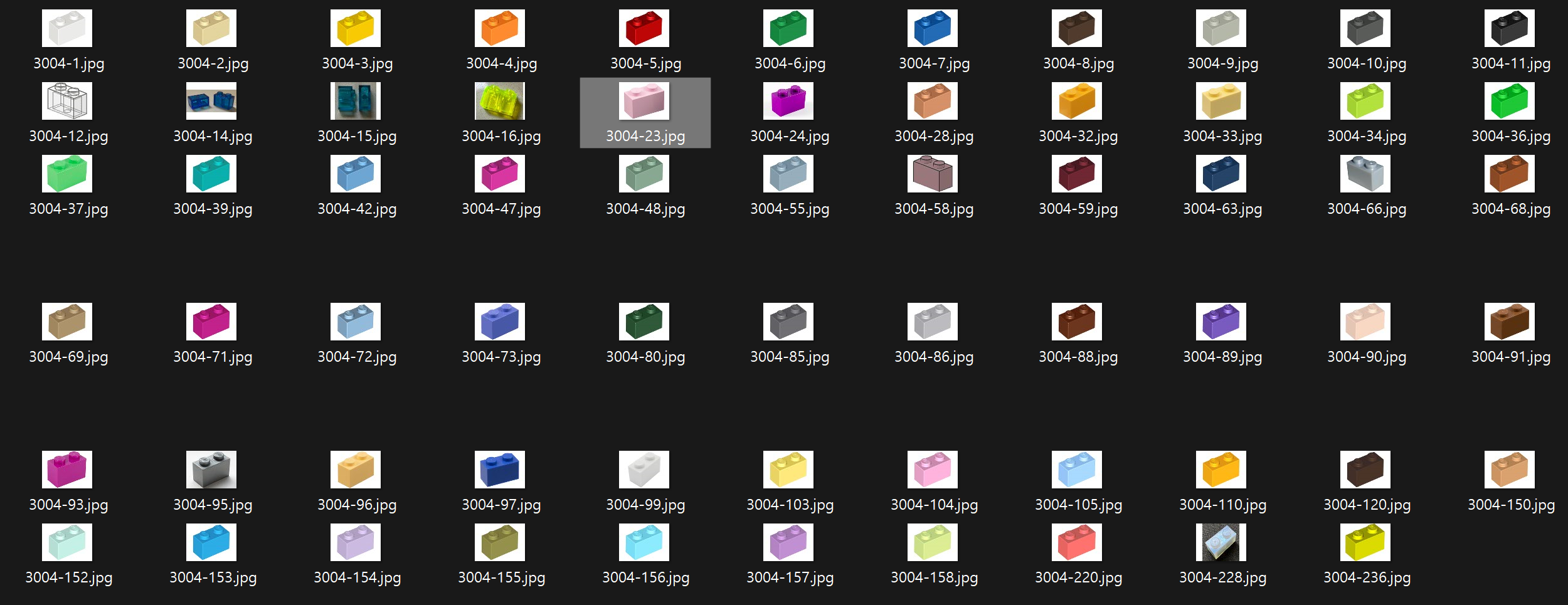
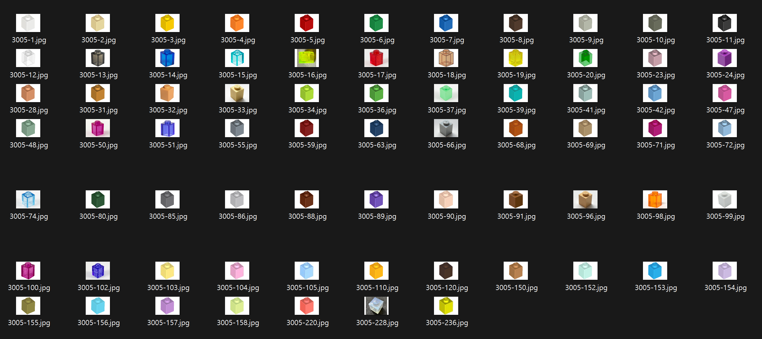
저번에 살펴봤던 bricklink 사이트를 좀 더 찾아보면서 img를 어떤 식으로 처리하는지 확인하고 자동으로 다운로드 받는 코드를 작성했습니다.

import requests
from bs4 import BeautifulSoup
import os

headers = {
    'User-Agent': 'Mozilla/5.0 (Windows NT 10.0; Win64; x64) AppleWebKit/537.36 (KHTML, like Gecko) Chrome/58.0.3029.110 Safari/537.3'
}

PART_ID = 3004
LIST_LEN = 300
OK = 200

# 이미지를 저장할 디렉터리 경로
image_folder = f'brick-data/pi-{PART_ID}'

# 디렉터리가 없으면 생성
if not os.path.exists(image_folder):
    os.makedirs(image_folder)

for idx in range(LIST_LEN):

    # 브릭 이미지 API
    image_url = f'https://img.bricklink.com/ItemImage/PT/{idx}/{PART_ID}.t1.png' 

    # HTTP 요청 보내기
    response = requests.get(image_url, headers=headers)

    # 응답 코드 확인
    if response.status_code == OK:  # 응답 코드가 200 (OK)일 때만 이미지를 저장
        # 이미지 다운로드
        image_data = response.content
                
        # 이미지를 브릭 ID로 저장
        image_path = os.path.join(image_folder, f'{PART_ID}-{idx}.jpg')
        with open(image_path, 'wb') as f:
            f.write(image_data)
    else:
        print(f"Failed to download image: {idx}, Status code: {response.status_code}")


print(f'Images saved to {image_folder}')

PART_ID에는 원하는 부품의 번호를 넣습니다. 아직 부품은 종류별로 하나씩만 이미지를 모으게 해놓았고 추가적으로 자동화 하지는 않았습니다. 이미지를 받았지만 비슷한 구도에 색깔만 다른 것들이 많아 그다지 학습이 잘 이루어질 것 같지는 않습니다.

3004

3005

일단 sklearn으로 모델을 만들고 학습을 시켜봅시다.

import os
import pickle

from skimage.io import imread
from skimage.transform import resize
import numpy as np
from sklearn.model_selection import train_test_split
from sklearn.model_selection import GridSearchCV
from sklearn.svm import SVC
from sklearn.metrics import accuracy_score

# prepare data
input_dir = './brick-data'
categories = ['3004', '3005']

data = []
labels = []

for cat_idx, category in enumerate(categories):
    for file in os.listdir(os.path.join(input_dir, f'pi-{category}')):
        img_path = os.path.join(input_dir, f'pi-{category}', file)
        print(img_path)
        img = imread(img_path)
        img = resize(img, (80, 60))
        data.append(img.flatten())
        labels.append(cat_idx)

data = np.asarray(data)
labels = np.asarray(labels)

# train / test split
x_train, x_test, y_train, y_test = train_test_split(
    data, labels,
    test_size=0.2,
    shuffle=True,
    stratify=labels
)

# train classifier
classifier = SVC()

parameters = [
    {
        'gamma': [0.01, 0.001, 0.0001], 
        'C': [1, 10, 100, 700]
    }
]

grid_search = GridSearchCV(classifier, parameters)

grid_search.fit(x_train, y_train)

# test performance
best_estimator = grid_search.best_estimator_

y_pred = best_estimator.predict(x_test)

score = accuracy_score(y_pred, y_test)

print(f'{score * 100}% of samples were correctly classified')

pickle.dump(best_estimator, open('./classifier.p', 'wb'))

분류 모델로는 Support Vector Classification을 썼습니다. 주어진 데이터를 가장 잘 나누는 결정 경계를 찾아줍니다. 기본적으로는 이진 분류 모델인데, 중첩해서 다중 분류도 되도록 만들 수는 있습니다.

C값은 오류에 대한 패널티입니다. 이 값이 작을수록 학습 데이터를 벗어나더라도 좀 더 관대하게 학습할 수 있고, 값이 커질수록 학습 데이터를 더 정확하게 학습합니다. 실제 C = 1000을 넣어버리니 학습 정확도가 100%가 나와버립니다. 가뜩이나 학습 데이터의 양도 적고 다양하다 할 수도 없으니 이건 과적합되었을 가능성이 매우 높습니다. 학습에서 썼던 데이터에 너무 초점이 맞춰져서 실제 추론을 위한 데이터를 받으면 제대로 된 답을 내지 못할 수 있습니다.

c700

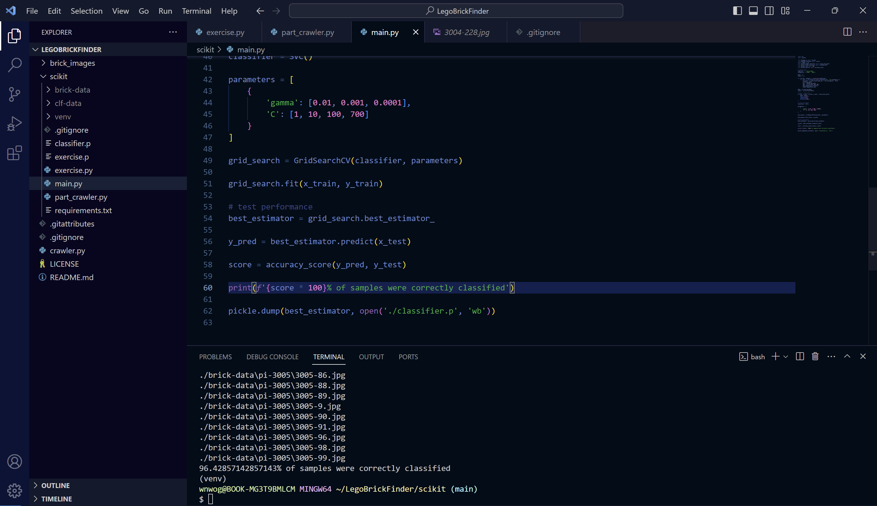
대략 700 정도 넣으니 정확도가 96%입니다. 근데 이 값도 채 100장이 되지 않는 학습 데이터에 대해서는 들쭉날쭉합니다. 충분히 학습되었다 말할 수 있으려면 더 많은 데이터가 필요할 것 같네요.

다음번엔 세 종류 이상의 분류 모델을 만들어야겠습니다.

Categories